Alpha Institute for Advanced Studies

This is a neat solution, and I we can proceed to writing up UFT399, followed by a review paper UFT400.

Complete Expression for the Spin Connection
To: Myron Evans <myronevans123>

This procedure seems to be unnecessisarily complicated. We have

<E(vac)> = <E(vac)>(2) + <E(vac)>(4) + …
and
<phi(vac)> = <phi(vac)>(2) + <phi(vac)>(4) + …

With

bold <E(vac)> = bold omega <phi(vac)>

it follows directly

omega_X = <E_X(vac)> / <phi(vac)> = (<E_X(vac)>(2) + <E_X(vac)>(4) + …) / (<phi(vac)>(2) + (<phi(vac)>(4) + …)

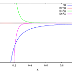
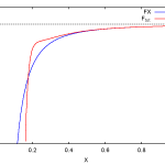
For the oscillatory example it follows that all degrees of derivatives only differ by a factor of k, and evaluating the above equation gives

omega_X = k * tan(k*X)

to all degrees of approximation.

Horst

Am 27.01.2018 um 14:13 schrieb Myron Evans:

This note completes Note 399(2) by calculating the complete spin connection components, exemplified by the X component. It is shown that all orders of <delta r dot delta r> can be eliminated so there is no need to calculate them explicitly, despite the fact that they are the basis for the theory. Infinities in the spin connection mean that the vacuum can transfer infinite amounts of energy to a well designed circuit. The complexity of the tensor Taylor series is no problem when computer algebra is used. So UFT399 can be written up on the basis of these three notes and the work completed by Horst for Section 3. Note that the vacuum being considered is the Lamb shift vacuum.

Many thanks, this is a very useful analysis and can of course go into Section 3.It is a matter of building a circuit to engineer the spin connection. Presumably this had been done prior to 2005 by the Alex hill group, and UFT311, UFT321, UT364, UFT382 and UFT383 engineer the spin connection in a sense. There has been a tremendous advance since 2005 and the patented and reproducible circuit details are in the public domain. The simpler the better and one can choose the simpler spin connection. So the lamb shift theory has been used to produce infinite energy in the form of a resonance.

Subject: Re: 399(1): Spin Connection Resonance from The Vacuum Fluctuations of the Lamb Shift
To: Myron Evans <myronevans123>

I checked the solutions of the diff.eq.(13). If the solution is real or complex (and oscillating) depends on the sign of the term omega_1*omega_X. Here it gives a real solution, see eq. %o3 of the protocol. Inserting an oscillatory form (%o6) does not solve the equation.

I continued with solution %o4. Inserting this into eq.(9) gives %o9 and – evaluated – %o11. The solution for phi_0 is %o12. This is a function increasing exponentially in time. It follows from the chosen omega_x which is decreasing in time but increasing in space. With this special form of the spin connection, it is possible to obtain infinite energy from the vacuum. However it will not be easy to construct such a spin connection, additional info on how to do this is required.

However it is possible to repeat the caculation with a simplified function (without space dependence)

omega_x = omega_0*exp(-omega_1*t).

Then a modulation in space is not requrired. This means, an exponentially decreasing omega can produce infinite energy. Maybe this means that spacetime curvature is converted to energy.

Horst

Am 22.01.2018 um 14:39 schrieb Myron Evans:

This note shows that in ECE2 theory vacuum fluctuations can produce an infinite potential energy by spin connection resonance, a subject which was initiated in 2005 at the request of civilians working for the U. S Navy who had acted as observers for an Alex Hill circuit that produced a giant surge of power from the vacuum. Since then the subject has been developed a great deal, especially in papers by Horst Eckardt and Doug Lindstrom. The Lamb shift is of course well described and it is is very likely that infinite power can be obtained from the vacuum through the well known Euler Bernoulli equation. The source term for the power is the vacuum electric field, so the circuit is tuned to maximize power. An elegant example of this is given in UFTt311, also see UFT321, add UFT382 and UFT383. The Alex Hill demonstration caused the hard headed U. S. Navy to go into resonance.

399(1).pdf

This is indeed a remarkable result by Horst, producing infinities in the spin connection starting again with the well known ideas of the Lamb shift theory. If there infinities in the spin connection the electric field strength also becomes infinite.

Date: Fri, Jan 26, 2018 at 2:29 PM
Subject: Re: 399(2): Ratio of Vacuum electric field to vacuum potential
To: Myron Evans <myronevans123>

This method of determining omega gives interesting results. I used an oscillating charge density rho(x) in one dimension:

rho(x) = rho_0 * cos(k*x).

Then the equations are simple enough to be solved analytically (see protocol). If all integration constants are set to zero, the result is

omega_x = k * tan(k*x),

see %o11 in the protocol. That means we have infinities in the spin connection, quite remarkable.
This result was obtained by computing E/phi. If the second method del^2 E / del^2 phi is used, the same result comes out, this time without integration constants that vanish due to two-fold differentiation (see %o13).

Horst

Am 24.01.2018 um 13:11 schrieb Myron Evans:

This note gives the useful new equations (20) to (22) so the spin connections can be found without having to know < delta r dot delta r >. The Poisson equation (24) can be used to find the potential in the absence of the vacuum for a given material charge density. This uses the highly developed methods of solution of the Poisson equation. %This method can be used in any area of physics, because the Poisson equation occurs throughout physics. It would be very interesting to graph the three spin connection components of Eqs. (20) to(22) for typical solutions of the Poisson equation. This calculation is given at second order, but can be extended to higher orders.

399(2).pdf

Many thanks, this is a most interesting result, indicating that the Lamb shift would change considerably for a small radiation volume.

Re: 398(5): Calculation of higher order <delta r dot delta r>
To: Myron Evans <myronevans123>

I calculated the expressions <dr*dr^2> and <ddr_dr^3> for several volumes. With
V = 4/3 pi a_0^3
(section 3 of protocol) the 6th order terms are even larger than the 4th order terms. When the radius values of 1s, 2s, 3s functions are inserted, this changes for the 2s and 3s fluctuations (section 4).

Horst

Am 18.01.2018 um 13:25 schrieb Myron Evans:

As can be seen, the theory gives reasonable results, and is based on Eq. (21), which gives an accurate description of the Lamb shift by summing over vacuum modes. Bethe’s calculation used quantum electrodynamics, which the ECE School of Thought rejects as a "dippy theory" in Feynman’s own words or an ugly theory" in Dirac’s words. Ryder sums up QED as follows "There is a feeling that there must be a better way of doing things", or similar ("Quantum Field Theory"). Accuracy in QED is obtained only by adjusting parameters, it is not magically hyperaccurate. These are given names like "virtual particles" (unobservables), dimensional regularization, renormalization and so on. In QCD things get dippier and stickier, and completely obscure and hyper complicated. The opposite of Ockham’s Razor. In a non dippy theory the infinities cannot be removed by magic. The higher order corrections in this theory depend on the radiation volume V. In a nuclear theory V can get to be very small, meaning that the higher order terms may dominate.

398(5).pdf

This note gives the useful new equations (20) to (22) so the spin connections can be found without having to know < delta r dot delta r >. The Poisson equation (24) can be used to find the potential in the absence of the vacuum for a given material charge density. This uses the highly developed methods of solution of the Poisson equation. %This method can be used in any area of physics, because the Poisson equation occurs throughout physics. It would be very interesting to graph the three spin connection components of Eqs. (20) to(22) for typical solutions of the Poisson equation. This calculation is given at second order, but can be extended to higher orders.

a399thpapernotes2.pdf

As can be seen, the theory gives reasonable results, and is based on Eq. (21), which gives an accurate description of the Lamb shift by summing over vacuum modes. Bethe’s calculation used quantum electrodynamics, which the ECE School of Thought rejects as a "dippy theory" in Feynman’s own words or an ugly theory" in Dirac’s words. Ryder sums up QED as follows "There is a feeling that there must be a better way of doing things", or similar ("Quantum Field Theory"). Accuracy in QED is obtained only by adjusting parameters, it is not magically hyperaccurate. These are given names like "virtual particles" (unobservables), dimensional regularization, renormalization and so on. In QCD things get dippier and stickier, and completely obscure and hyper complicated. The opposite of Ockham’s Razor. In a non dippy theory the infinities cannot be removed by magic. The higher order corrections in this theory depend on the radiation volume V. In a nuclear theory V can get to be very small, meaning that the higher order terms may dominate.

a398thpapernotes5.pdf

The usual result for the Lamb shift, the universal constant shift Eq. (24), is modified to Eq. (25), in which there appear classical, non constant, corrections to the famous calculation. These can be worked out with computer algebra and graphed. Inverse powers of the radiation volume appear in each term. So for small radiation volumes the correction may dominate, leading to entirely new spectral predictions.

a398thpapernotes3.pdf

This is given by Eq. (17) from which the vector spin connection may be computed. The usual dipole magnetic flux density is given by Eq. (10), which is broken out into its three scalar Cartesian components in Eqs. (11) to (13). The tensor Taylor series is applied to each component. ECE2 theory automatically gives the vacuum correction through the definition (3). The standard model fails completely to account for the vacuum field because it defines the magnetic flux density using equation (2), without the spin connection. Clearly this calculation is impractical by hand, but straightforward by computer algebra, using the program written by Horst for isotropic averaging. The tensor Taylor expansion is very fundamental and general and can be applied throughout the natural sciences and engineering to research the effect of the vacuum on physics. I expect that the graphics for this calculation will display hitherto unknown patterns due to the vacuum. The computation can be carried out in any coordinate system, not just Cartesian.

a396thpapernotes4.pdf

I would say that the complete delta F term on the right hand side of equation (7) of Note 396(3) must be equated to the complete sum of the binomial expansion. They cannot be equated term by term. However, for v << c Eq. (16) holds, in which delta F is the sum of the fourth and sixth order corrections that you have already worked out, plus higher order terms. The reasoning is that the lagrangian (10) is known to give precession, (UFT377) so if the vacuum correction delta F is equated to the right hand side of Eq. (16), delta F will give the same precession. Therefore precession originates in the vacuum, QED.

Very interesting results again, the fundamental tensor Taylor expansion shows that the vacuum influences the inverse square law. The method of Note 396(3) is still valid and it would be interesting if an orbit could be calculated directly from these new force laws. It would also be useful if the analytical expressions could be given for the fourth and sixth order corrections. in order to see how the isotropically averaged fluctuations contribute. The saddle in the inverse square law looks to be the key feature. Date: Thu, Jan 4, 2018 at 12:23 PM
Subject: Graphics of 4th and 6th order fluctuations in the 1/r^2 force law
To: Myron Evans <myronevans123>

The fluctuation terms have been computed for a fixed delta r value and graphed. We see that 4th order gives a repelling contribution which leads to a saddle in the force graph. For small r then the force is more attractive. May be an explanation for relativistic effects.

Horst

Am 04.01.2018 um 10:30 schrieb Myron Evans:

In this note the tensorial Taylor series (5) is used to calculate the change in the Hooke / Newton inverse square law due to the vacuum, and it is shown to second order that the orbital precession of UFT377 is due to the vacuum. It may be concluded that all precessions are due to the vacuum, or aether, or spacetime. This is a major discovery. The <delta r dot delta r > needed to induce orbital precession is given to second order in Eqs. (18) to (20). It would be very interesting to graph Eq. (5) to higher orders of the tensor Taylor series. Note carefully that the same tensor Taylor series is used in the theory of the Lamb shift in atomic H. So we achieve unification of concept in the description of atomic and orbital physics.